|
Getting your Trinity Audio player ready...
|
Master Excel’s math and trigonometry functions like MOD, ABS, ROUNDUP, SQRT, and RAND with real-life examples explained in simple language.
When working with numbers in Excel, knowing basic math functions can save you tons of time. From simple rounding to generating random numbers, Excel has a powerful set of Math and Trigonometry functions to handle daily tasks easily.
In this blog, we’ll go through each of these functions in a simple, easy-to-follow manner with real-life examples to help you understand when and how to use them.
1. MOD(): Get Remainder
Syntax: =MOD(number, divisor)
This function returns the remainder after dividing one number by another.
Example 1:
You have 23 students and want to divide them into groups of 5.
=MOD(23, 5) ➔ Result: 3 (5*4 = 20, so 23-20 = 3)
So, 3 students will remain without a full group.
2. ABS(): Get Absolute Value
Syntax: =ABS(number)
Returns the positive version of a number, removing any negative sign.
Example 2:
You’re comparing expected sales vs actual, and want the difference without considering the sign.
=ABS(A2 – B2)
This shows the sales difference as a positive number.
If A2 = 100, B2 = 300, then the result is -200. After ABS, the result is 200
3. INT(): Round Down to Whole Number
Syntax: =INT(number)
Rounds a number down to the nearest integer.
Example 3:
You’re calculating hours from minutes:
=INT(A2/60)
If A2 is 135, the result will be 2 full hours.
4. ROUNDUP(): Round Number Up
Syntax: =ROUNDUP(number, num_digits)
Always rounds the number up to the specified decimal places.
Example 4:
Shipping charges need to be rounded up to the next 10.
=ROUNDUP(A2, -1)
If A2 = 54, the result is 60.
5. ROUNDDOWN(): Round Number Down
Syntax: =ROUNDDOWN(number, num_digits)
Rounds the number down towards zero.
Example 5:
Truncating the price for a sale item:
=ROUNDDOWN(A2, 0)
If A2 = 99.9, the result is 99.
Read More: ROUND Function in Excel
6. POWER(): Raise Number to a Power
Syntax: =POWER(number, power)
Raises a number to a power (exponent).
Example 6:
Calculate compound growth:
=POWER(3, 2)
This gives the power of 3, that is 3*3 = 9.
Note: =POWER(2, 3) -> 2*2*2 = 8 (Result)
7. SQRT(): Square Root
Syntax: =SQRT(number)
Returns the square root of a number.
Example 7:
In engineering or geometry calculations:
=SQRT(A2)
If A2 = 144, the result is 12.
8. RAND(): Random Decimal Number
Syntax: =RAND()
Returns a random decimal between 0 and 1.
Example 8: Random Customer Feedback Ratings
You want to simulate random customer feedback ratings.
=RAND()*5
This gives a random value between 0 and 5.
9. RANDBETWEEN(): Random Integer
Syntax: =RANDBETWEEN(bottom, top)
Returns a random whole number between two numbers.
Example 9: Generate lucky draw winners:
=RANDBETWEEN(1, 100)
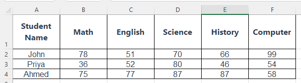
Example 9.1: Generate Random Marks for Students
Suppose you want to create a marksheet for students and generate random marks between 35 and 100 (passing to full marks) for 5 subjects.
| Student Name | Math | English | Science | History | Computer |
|---|---|---|---|---|---|
| John | =RANDBETWEEN(35,100) | =RANDBETWEEN(35,100) | =RANDBETWEEN(35,100) | =RANDBETWEEN(35,100) | =RANDBETWEEN(35,100) |
| Priya | =RANDBETWEEN(35,100) | =RANDBETWEEN(35,100) | =RANDBETWEEN(35,100) | =RANDBETWEEN(35,100) | =RANDBETWEEN(35,100) |
| Ahmed | =RANDBETWEEN(35,100) | =RANDBETWEEN(35,100) | =RANDBETWEEN(35,100) | =RANDBETWEEN(35,100) | =RANDBETWEEN(35,100) |
Sample Data:
💡 Explanation:
RANDBETWEEN(35,100)generates a random integer between 35 and 100.- This is useful when creating sample data for a demo, practice, or testing formulas like average, grade calculation, etc.
10. CEILING(): Round Up to Nearest Multiple
Syntax: =CEILING(number, significance)
Rounds number up to the nearest multiple of significance.
Example 10:
Round salary to the next 500:
=CEILING(A2, 500)
If A2 = 3250, the result is 3500.
11. FLOOR(): Round Down to Nearest Multiple
Syntax: =FLOOR(number, significance)
Rounds the number down to the nearest multiple.
Example 11:
For discount thresholds:
=FLOOR(A2, 100)
If A2 = 849, the result is 800.
12. PRODUCT(): Multiply Numbers
Syntax: =PRODUCT(number1, [number2], ...)
Multiplies all numbers given.
Example 12:
Get total cost:
=PRODUCT(Price, Quantity)
If Price = 120 and Qty = 3, the result is 360.
13. PI(): Return Value of π
Syntax: =PI()
Returns the value of π (3.1415927)
Example 13:
Calculate the area of a circle:
=PI()*POWER(Radius,2)
Summary Table
| Function | Purpose |
|---|---|
| MOD() | Get the remainder of the division |
| ABS() | Absolute value |
| INT() | Round down to an integer |
| ROUNDUP() | Round number up |
| ROUNDDOWN() | Round number down |
| POWER() | Gives the power of a number |
| SQRT() | Square root |
| RAND() | Random decimal between 0 and 1 |
| RANDBETWEEN() | Random integer in range |
| CEILING() | Round up to the nearest multiple |
| FLOOR() | Round down to the nearest multiple |
| PRODUCT() | Multiply numbers |
| PI() | Return value of π |
FAQs
Q1: Can I use RAND or RANDBETWEEN for lotteries or actual selections?
Yes, but since they recalculate on every change, use Copy > Paste as Values to freeze results.
Q2: When should I use CEILING instead of ROUNDUP?
Use CEILING when you need to round to a specific multiple, like to the nearest 500 or 100.
Q3: What’s the difference between INT and ROUNDDOWN?INT always rounds down toward negative infinity, while ROUNDDOWN rounds toward zero.
Q4: Is POWER better than using ^ symbol?
Both work the same: =POWER(2,3) is the same as =2^3.
Final Thoughts
These functions may seem small, but they are mighty tools in your Excel toolkit. Whether you’re calculating, rounding, analyzing data, or creating random simulations, Math and Trig functions make your job easier, smarter, and more accurate.
Start practising them today, and your Excel skills will skyrocket!
What’s Next?
In the next post, we’ll learn about the 20 Other Useful Excel Functions