|
Getting your Trinity Audio player ready...
|
Data is powerful only when you can find and connect it effectively — and that’s where Lookup Functions in Zoho Sheets come in.
Whether you’re fetching employee details from another table, finding product prices, or matching IDs across multiple datasets, lookup formulas are the backbone of any spreadsheet-based data analysis.
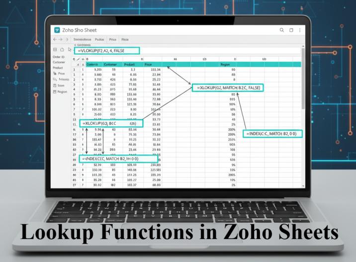
In this guide, we’ll learn about the most used lookup functions in Zoho Sheets — VLOOKUP, HLOOKUP, XLOOKUP, INDEX, MATCH, and their combinations — with real-life business scenarios, examples, and syntax.
1. Introduction to Lookup Functions
Lookup functions allow you to search a value in one part of your sheet and return related information from another column or row.
For example:
If you have an Employee ID and want to fetch the Employee Name or Department automatically — lookup functions make that possible.
Why Use Lookup Functions?
✅ Save time by avoiding manual search
✅ Reduce human errors
✅ Link related datasets (like Sales & Products tables)
✅ Make your reports and dashboards dynamic
Sample Dataset
Let’s use the following sample data throughout our examples:
| Employee ID | Employee Name | Department | Designation | Salary | Location |
|---|---|---|---|---|---|
| EMP001 | Priya Sharma | HR | HR Manager | 65000 | Delhi |
| EMP002 | Amit Patel | Finance | Accountant | 48000 | Mumbai |
| EMP003 | Neha Verma | IT | Developer | 75000 | Bangalore |
| EMP004 | Rohit Das | IT | Analyst | 72000 | Pune |
| EMP005 | Meena Joshi | Marketing | Marketing Head | 82000 | Chennai |
| EMP006 | Rakesh Singh | HR | Recruiter | 46000 | Delhi |
| EMP007 | Aarav Gupta | Finance | Sr. Accountant | 54000 | Mumbai |
| EMP008 | Sneha Rao | IT | Tester | 50000 | Hyderabad |
| EMP009 | Kiran Sahu | Sales | Sales Executive | 42000 | Raipur |
| EMP010 | Anjali Jain | Sales | Sales Manager | 70000 | Jaipur |
2. VLOOKUP Function in Zoho Sheets
Syntax:
=VLOOKUP(lookup_value, table_array, col_index, [is_sorted])
Parameters:
lookup_value: The value you want to search (e.g., Employee ID)table_array: The range containing datacol_index: The column number to return value fromis_sorted: UseFALSEfor exact match,TRUEfor approximate
Example 1: Find Employee Name by Employee ID
Formula:
=VLOOKUP("EMP004", A2:F11, 2, FALSE)
Result: Rohit Das
This searches column A for EMP004 and returns the corresponding value from column 2 (Employee Name).
Example 2: Dynamic VLOOKUP using Cell Reference
If Employee ID is entered in H2, and you want to display Department in I2:
=VLOOKUP(H2, A2:F11, 3, FALSE)
Now, when you change the Employee ID in H2, the Department updates automatically — perfect for interactive dashboards or forms.
Example 3: Error Handling with VLOOKUP
Sometimes the searched value might not exist. Combine VLOOKUP with IFERROR:
=IFERROR(VLOOKUP(H2, A2:F11, 2, FALSE), "Not Found")
If no match is found, it returns “Not Found” instead of showing an error.
Read More: How to use IFERROR & IFNA
Example 4: Lookup from Another Zoho Sheet (Cross-Sheet Lookup)
In real business use cases, your data is rarely stored in a single spreadsheet.
You might have:
- One Zoho Sheet with the Employee Master Data
- Another Zoho Sheet used for Payroll or Attendance
In such cases, you can link data across multiple Zoho Sheets using:
The IMPORTRANGE() function — just like in Google Sheets.
Syntax:
=IMPORTRANGE("spreadsheet_url", "range_string")
spreadsheet_url: The URL of the other Zoho Sheetrange_string: The specific range, e.g.,"Sheet1!A2:F11"
Example:
Let’s say your Employee Master Sheet has this link:
https://sheet.zoho.com/sheet/open/abcd12345
To import Employee ID and Salary columns, use:
=IMPORTRANGE("https://sheet.zoho.com/sheet/open/abcd12345", "EmployeeMaster!A2:E11")
This will pull the data into your current sheet.
Now, you can apply a VLOOKUP on the imported range like this:
=VLOOKUP(A2, IMPORTRANGE("https://sheet.zoho.com/sheet/open/abcd12345", "EmployeeMaster!A2:E11"), 5, FALSE)
Explanation:
A2→ Employee ID to searchIMPORTRANGE(...)→ Imports employee master data dynamically5→ Fetches value from the 5th column (Salary)FALSE→ Ensures exact match
Result: Displays the Salary of the employee even though the source data lives in another Zoho Sheet.
Real-Life Scenario: Multi-Branch Payroll System
Suppose you have:
- HR_Master.zohosheet (Employee master for all branches)
- Branch_Raipur.zohosheet (Branch-specific payroll)
In Branch_Raipur, you can import and connect to the master sheet using IMPORTRANGE()
Then, run:
=VLOOKUP(Employee_ID, ImportedRange, 5, FALSE)
to fetch Employee Salary, Department, or Designation — directly from the main HR file.
💡 This ensures consistency, centralization, and automation across multiple departments — a perfect setup for MIS or Data Analyst roles managing multi-sheet data.
Also Read: All About IMPORTRANGE Function
3. HLOOKUP Function
Syntax:
=HLOOKUP(lookup_value, table_array, row_index, [is_sorted])
HLOOKUP works horizontally — it searches in the first row and returns a value from the same column in a specified row.
Example 1: Get Employee Name using Horizontal Table
| Data Type | EMP001 | EMP002 | EMP003 |
|---|---|---|---|
| Name | Priya Sharma | Amit Patel | Neha Verma |
| Department | HR | Finance | IT |
| Salary | 65000 | 48000 | 75000 |
Formula:
=HLOOKUP("EMP002", A1:D4, 3, FALSE)
Result: 48000
This looks for EMP002 in row 1 and returns the corresponding salary from row 3.
Example 2: HLOOKUP with IFERROR
=IFERROR(HLOOKUP(H2, A1:D4, 2, FALSE), "Not Available")
If employee code isn’t found, it will display a clean message instead of an error.
4. XLOOKUP Function (The Modern Replacement)
Zoho Sheets supports XLOOKUP, which simplifies lookup operations — it replaces both VLOOKUP and HLOOKUP.
Syntax:
=XLOOKUP(lookup_value, lookup_array, return_array, [if_not_found])
Example 1: Find Department by Employee Name
=XLOOKUP("Amit Patel", B2:B11, C2:C11, "Not Found")
Result: Finance
It searches for Amit Patel in column B and returns the corresponding department from column C.
Example 2: XLOOKUP with Cell Reference
If user types the employee name in H2, use:
=XLOOKUP(H2, B2:B11, D2:D11, "Not Found")
Returns the designation dynamically.
Example 3: XLOOKUP with Nested Calculation
Want to calculate bonus = Salary * 10% of the employee entered in H2?
=XLOOKUP(H2, B2:B11, E2:E11, 0) * 10%
5. INDEX + MATCH Combination
Before XLOOKUP, advanced users preferred INDEX and MATCH because they were more flexible than VLOOKUP.
Syntax:
=INDEX(return_range, MATCH(lookup_value, lookup_range, 0))
Example 1: Get Designation by Employee ID
=INDEX(D2:D11, MATCH("EMP005", A2:A11, 0))
Result: Marketing Head
MATCH finds the position of EMP005, and INDEX returns value from the same row in Designation column.
Example 2: Use Cell Reference for Flexibility
=INDEX(E2:E11, MATCH(H2, A2:A11, 0))
If H2 contains EMP008, result → 50000 (Salary).
Example 3: INDEX + MATCH for Two-Way Lookup
Suppose you have this table:
| Metric | Jan | Feb | Mar |
|---|---|---|---|
| Sales | 12000 | 15000 | 17000 |
| Profit | 3000 | 4000 | 4200 |
If you want to find the Profit for Feb, use:
=INDEX(B2:D3, MATCH("Profit", A2:A3, 0), MATCH("Feb", B1:D1, 0))
Result: 4000
This is a two-dimensional lookup — finds row by “Profit” and column by “Feb”.
6. Real-Life Scenarios Using Lookup Functions
Let’s understand how these formulas help in practical, day-to-day data analysis.
Scenario 1: Salary Slip Generator
In a payroll dashboard:
- Employee ID is entered in cell H2
- You want to fetch Name, Designation, Department, and Salary automatically:
=XLOOKUP(H2, A2:A11, B2:B11, "Not Found")  → Name
=XLOOKUP(H2, A2:A11, D2:D11, "Not Found")  → Designation
=XLOOKUP(H2, A2:A11, C2:C11, "Not Found")  → Department
=XLOOKUP(H2, A2:A11, E2:E11, "Not Found")  → Salary
This makes your salary slip creation or employee information retrieval automated.
Scenario 2: Sales Dashboard Linking
You have two sheets —
Sheet1: Product-wise sales
Sheet2: Product master with price and category
Using:
=VLOOKUP(A2, ProductMaster!A2:C100, 3, FALSE)
You can link product codes to categories or pricing details dynamically.
Scenario 3: Region-Wise Reporting
If you maintain regional data across multiple sheets:
=INDIRECT("'"&H2&"'!B2:B50")
can dynamically fetch values from the sheet name entered in H2.
This, combined with INDEX-MATCH or XLOOKUP, enables multi-region reports easily.
7. Comparing Lookup Functions
| Function | Direction | Supports Left Lookup | Dynamic Range | Simplicity | Recommended |
|---|---|---|---|---|---|
| VLOOKUP | Vertical | ❌ No | ❌ Static | Easy | Beginners |
| HLOOKUP | Horizontal | ❌ No | ❌ Static | Easy | Rarely used |
| XLOOKUP | Both | ✅ Yes | ✅ Yes | Very Easy | ✅ Modern & Preferred |
| INDEX + MATCH | Both | ✅ Yes | ✅ Yes | Moderate | ✅ Advanced Users |
8. Best Practices
✅ Always use absolute references ($A$2:$F$11) when copying formulas.
✅ Combine with IFERROR() for cleaner results.
✅ Prefer XLOOKUP for flexibility and performance.
✅ Use INDEX+MATCH when working with large datasets or older systems.
✅ Avoid sorted lookup unless you know your dataset is properly sorted.
Conclusion
Lookup functions are the core tools for data professionals using Zoho Sheets.
They help connect different tables, automate report generation, and simplify analysis — all without writing a single line of code.
From VLOOKUP to XLOOKUP and INDEX-MATCH, mastering these formulas will help you handle everything from MIS reporting to real-time dashboards efficiently.
In the next post, we’ll cover “Text & String Manipulation Functions in Zoho Sheets” — to clean, transform, and combine data smartly.
What’s Next?
In the next post, we’ll learn about the Advanced Functions in Zoho Sheets like CHOOSE, FILTER, QUERY, INDIRECT