|
Getting your Trinity Audio player ready...
|
Learn how to use the CHOOSE function in Excel with easy explanations and practical real-life examples. Ideal for decision making, conditional logic, and dynamic value selection.
Microsoft Excel is packed with functions that help you automate tasks, calculate data, and make decisions. One such powerful yet underrated function is the CHOOSE function. Whether you’re selecting items based on numbers, building dashboards, or working with lookup alternatives, CHOOSE can be a smart tool in your formula toolbox.
In this guide, we’ll break down the CHOOSE function in detail, explain how it works, and explore real-life use cases.
What is the CHOOSE Function?
The CHOOSE function returns a value from a list based on a given position number (index).
Syntax:
=CHOOSE(index_num, value1, [value2], …)
- index_num – The position of the value you want to return.
- value1, value2, … – A list of values from which one will be chosen.
Simple Example:
=CHOOSE(2, “Apple”, “Banana”, “Cherry”)
Returns: Banana (because it’s the 2nd item in the list)
Why Use CHOOSE Function?
- Easy alternative to nested IFs or SWITCH
- Simplifies category selection
- Can be used in combination with MATCH, RANDBETWEEN, and others
- Great for generating random items or static lookup lists
Real-Life Examples
Example 1: Return Day Name from Number
=CHOOSE(A1, “Sunday”, “Monday”, “Tuesday”, “Wednesday”, “Thursday”, “Friday”, “Saturday”)
If A1 = 3 → returns: Tuesday
Useful when converting weekday numbers to names manually.
Example 2: Select a Shipping Method Based on Code
| Code | Method |
|---|---|
| 1 | Standard |
| 2 | Express |
| 3 | Overnight |
=CHOOSE(B2, “Standard”, “Express”, “Overnight”)
If B2 = 2 → returns: Express
Example 3: Generate Random Fruit
=CHOOSE(RANDBETWEEN(1, 4), “Apple”, “Banana”, “Mango”, “Orange”)
Returns a random fruit name every time the sheet recalculates.
Example 4: Use with MATCH to Create Static Lookup
Suppose your data is limited and doesn’t change much. Instead of using VLOOKUP:
=CHOOSE(MATCH(“C”, {“A”,”B”,”C”}, 0), 100, 200, 300)
Returns: 300
Also Read: Match Function in Excel
Example 5: Monthly Bonus Based on Rank
| Rank | Bonus Formula |
| 1 | 5000 |
| 2 | 3000 |
| 3 | 2000 |
| >3 | 1000 |
=IF(A2>3, 1000, CHOOSE(A2, 5000, 3000, 2000))
If A2 = 2 → returns: 3000
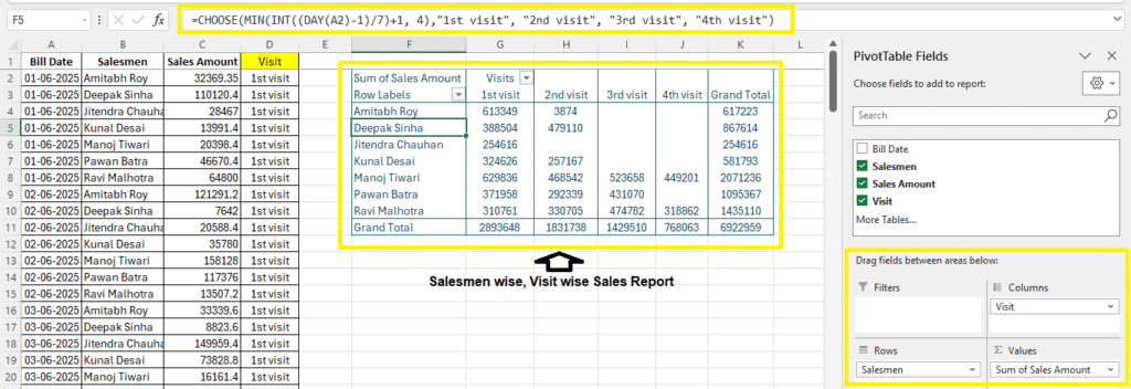
Example 6: Determine Visit Based on Date of the Month
Let’s say column P contains sales visit dates. You want to classify visits into the 1st to 4th visit of the month:
=CHOOSE(MIN(INT((DAY(P2)-1)/7)+1, 4), “1st Visit”, “2nd Visit”, “3rd Visit”, “4th Visit”)
👉 This ensures even if the day is beyond 28th (e.g., 29–31), it still falls under “4th Visit” due to MIN()
Also Read: Excel MIN & MAX Functions
Note: The INT Function is used to convert a decimal number to the nearest lower whole number (i.e., it always rounds down to the nearest whole number).
You can use this formula to create a Pivot Table that shows total sales by salesmen and visit-wise categories like:
| Salesman | 1st Visit | 2nd Visit | 3rd Visit | 4th Visit | Grand Total |
| Amitabh Roy | 613349 | 374 | 617223 | ||
| Deepak Sinha | 388504 | 47910 | 867614 | ||
| Jitendra Chauhan | 254616 | 254616 | |||
| Kunai Desai | 324626 | 257167 | 581793 | ||
| Manoj Tiwari | 629836 | 468542 | 523658 | 449201 | 2071236 |
| Pawan Batra | 371958 | 292339 | 431070 | 1095367 | |
| Ravi Malhotra | 310761 | 330705 | 474782 | 318862 | 6922959 |
Read More: Pivot Table in Excel
Download Practice File
Limitations of CHOOSE
- Index must be numeric (can’t use text)
- Maximum of 254 values can be passed
- Static values only — dynamic lists require other functions
Pro Tips
- You can return formulas or ranges using CHOOSE:
=SUM(CHOOSE(A1, B2:B5, C2:C5)) - Combine with INDIRECT if list is stored as named ranges
- CHOOSE is faster than nested IFs in many scenarios
Summary Table
| Task | Formula Example | Result |
| Day from number | =CHOOSE(3, “Sun”, “Mon”, “Tue”) | Tue |
| Lookup from code | =CHOOSE(B2, “Std”, “Exp”, “O/N”) | Based on B2 |
| Static lookup via MATCH | =CHOOSE(MATCH(“C”, {“A”,”B”,”C”}, 0), 100, 200, 300) | 300 |
| Conditional bonus | =IF(A2>3, 1000, CHOOSE(A2, 5000, 3000, 2000)) | Based on rank |
| Week of month from date | =CHOOSE(MIN(INT((DAY(P2)-1)/7)+1,4), “1st Visit”, “2nd Visit”, “3rd Visit”, “4th Visit”) | 1st–4th Visit |
FAQs – CHOOSE Function in Excel
Is CHOOSE better than IF?
For small lists, yes. CHOOSE is cleaner and shorter than multiple IFs.
Does CHOOSE work with named ranges?
Yes, especially if you're referencing arrays or columns.
Final Thoughts
The CHOOSE Function is an elegant solution for simple list lookups, replacements, and control structures. While it doesn’t replace more powerful tools like VLOOKUP or INDEX & MATCH, it shines when you’re dealing with static, short, and predictable lists. Combine it with other Excel functions, and you’ve got a lightweight, smart solution for many problems.
Start using CHOOSE today — and make your Excel sheets simpler, smarter, and cleaner!
What’s Next?
In the next post, we’ll learn about the Math and Trigonometry Functions in Excel