|
Getting your Trinity Audio player ready...
|
Learn Conditional Formatting in Excel from beginner to advanced level with real-life examples. Highlight data automatically using rules, formulas, and visuals.
Conditional Formatting in Excel allows you to automatically apply formatting—such as colors, icons, or bold text—based on the values in your spreadsheet. Whether you’re tracking sales, highlighting top customers, or flagging low inventory, this tool helps visualize your data clearly.
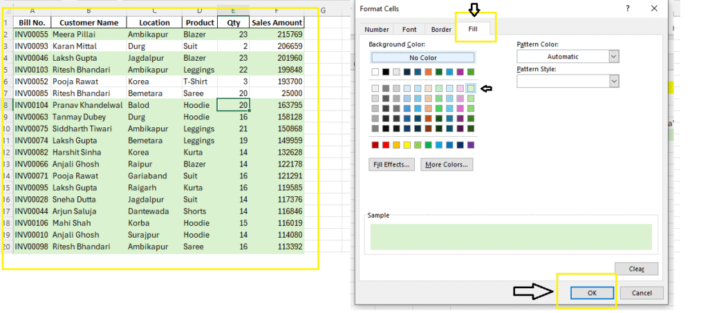
We’ll use the following Sales Data Table as our reference for examples:
| Bill No. | Customer Name | Location | Product | Qty | Sales Amount |
|---|---|---|---|---|---|
| INV0030 | Yuvraj Nair | Korba | Suit | 6 | 13991 |
| INV0033 | Yuvraj Nair | Rajnandgaon | T-Shirt | 9 | 64800 |
| INV0081 | Yuvraj Nair | Gariaband | T-Shirt | 3 | 28467 |
| INV0020 | Vivek Malhotra | Balod | Suit | 6 | 41580 |
| INV0058 | Vivaan Sharma | Sarguja | Kurta | 4 | 46670 |
| … | … | … | … | … | … |
Basic Conditional Formatting Examples
1. Highlight Sales Greater Than ₹40,000
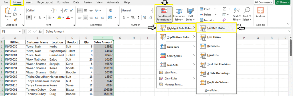
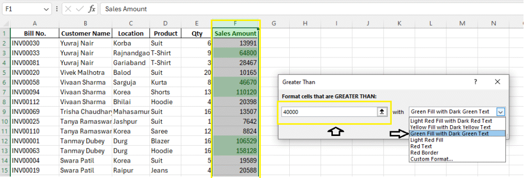
Highlight all sales where the Sales Amount > 40000.
- Select the “Sales Amount” column.
- Go to Home > Conditional Formatting > Highlight Cell Rules > Greater Than.
- Enter
40000and choose a highlight color (e.g., light green).
2. Highlight Duplicate Customer Names
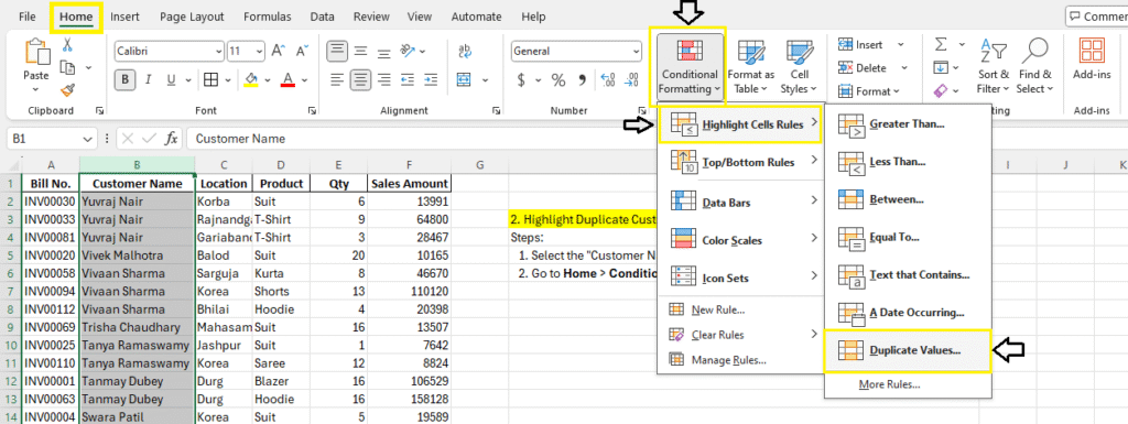
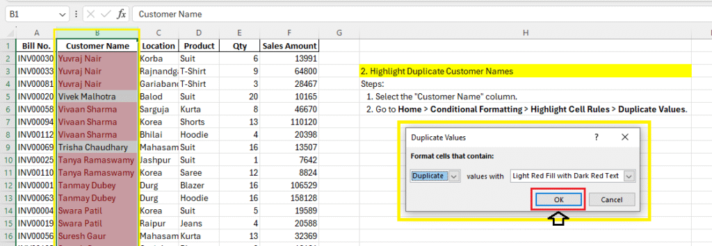
- Select the “Customer Name” column.
- Go to Home > Conditional Formatting > Highlight Cell Rules > Duplicate Values.
3. Color Scale Based on Qty
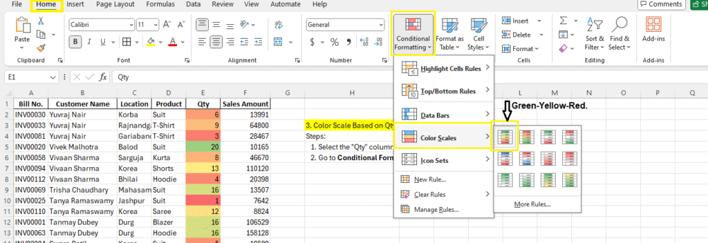
Visualize purchase volume with a color gradient.
- Select the “Qty” column.
- Go to Home > Conditional Formatting > Color Scales > Green-Yellow-Red.
Intermediate Examples
4. Highlight Top 3 Highest Sales
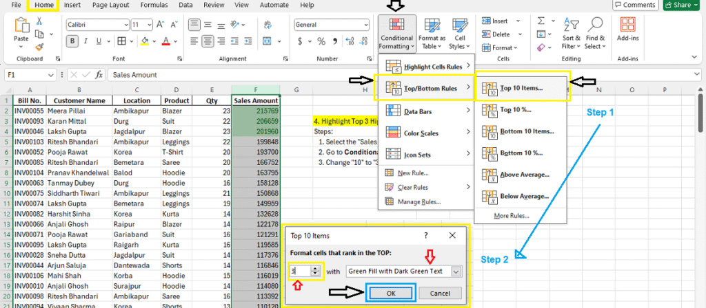
- Select the “Sales Amount” column.
- Go to Conditional Formatting > Top/Bottom Rules > Top 10 Items.
- Change “10” to “3” and apply bold red fill.
5. Highlight Customers with Hoodie Orders
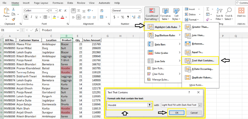
Use a text match to highlight Hoodie product rows.
- Select the “Product” column.
- Go to Conditional Formatting > Highlight Cell Rules > Text that Contains > Type “Hoodie”
6. Highlight Sales from Gariaband
- Select the “Location” column.
- Use “Text that Contains” with value “Gariaband”
Advanced Examples
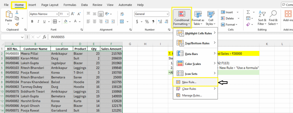
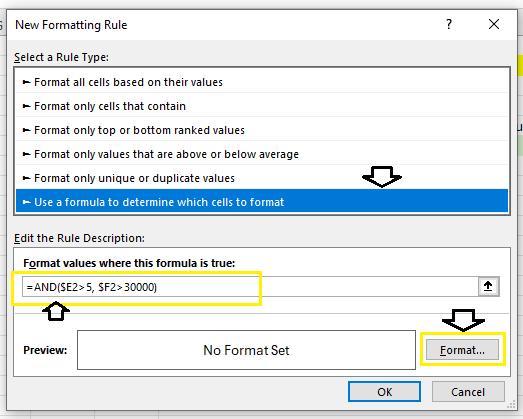
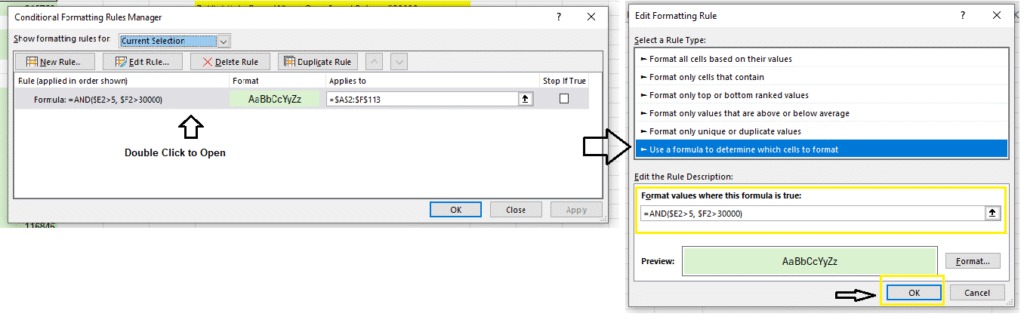
7. Highlight Rows Where Qty > 5 and Sales > ₹30000
Use a formula to apply formatting across the row.
- Select entire data range (e.g., A2:F113)
- Go to Conditional Formatting > New Rule > “Use a formula”
=AND($E2>5, $F2>30000)
Also Read: How to use AND & OR in Excel
8. Color Sales Over Average Using Formula
=F2>AVERAGE($F$2:$F$20)
Highlights sales amounts above the average.
9. Highlight All Hoodie Orders with Qty < 5
=AND($D2=”Hoodie”, $E2<5)
10. Highlight Sales from Specific Customers
=OR($B2=”Yuvraj Nair”, $B2=”Tanmay Dubey”)
Real-Life Use Cases from the Table
- Highlight all Hoodie orders with red if Qty < 5
- Use a color scale to show which cities have highest total sales
- Apply icon sets to the “Sales Amount” column
- Flag duplicate orders using “Bill No.”
- Identify VIP customers (Sales > ₹50,000)
Clear Rules
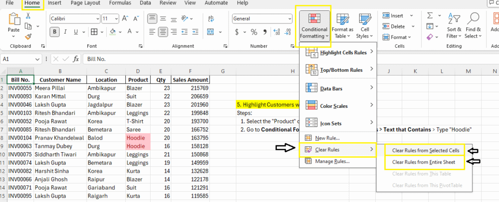
To remove conditional formatting:
- Select the data range or sheet.
- Go to Home > Conditional Formatting > Clear Rules.
- Choose from:
- “Clear Rules from Selected Cells”
- “Clear Rules from Entire Sheet”
This helps when rules overlap or no longer apply.
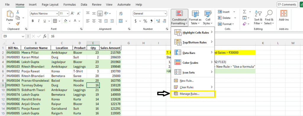
Manage Rules
You can view, edit, or delete rules:
- Go to Home > Conditional Formatting > Manage Rules.
- The Conditional Formatting Rules Manager will appear.
- You can:
- View all rules in the current worksheet or selection
- Change the formula or formatting
- Delete or reorder rules
Managing rules is essential for maintaining complex formatting.
Best Practices
- Use relative vs. absolute references correctly
- Keep rules organized using Manage Rules
- Avoid too many formatting rules—they can slow performance
- Use named ranges for dynamic tables
Download Practice Material
Summary
Conditional Formatting is a smart way to highlight trends, patterns, and outliers in your Excel data. With the right formulas, you can make even complex logic easy to visualize.
FAQs – Conditional Formatting in Excel
Can I apply more than one rule?
Yes, use Manage Rules to adjust priority.
Will it work in Excel Online?
Yes, most rules are supported but formula-based ones may be limited.
Does it update automatically with new data?
Yes, if applied on a Table or dynamic range.
What’s Next?
In the next post, we’ll learn about the Data Validation in Excel