Excel Functions to Handle Text

Learn how to use Excel functions to handle text like LEFT, RIGHT, MID, FIND, SEARCH, LEN, and TEXT to extract, format, and analyze text with real-life examples.

Summary Table: Excel Functions to Handle Text

Function	Purpose
LEFT	Extract characters from the beginning of text
RIGHT	Extract characters from the end of text
MID	Extract characters from the middle of text
FIND	Find position of text (case-sensitive)
SEARCH	Find position of text (case-insensitive)
LEN	Count total number of characters
TEXT	Format numbers or dates as text

---

Introduction

When working with text data in Excel—like names, product codes, emails, or dates—text functions become essential tools for cleaning, formatting, and extracting information. This guide covers 7 key functions from beginner to advanced levels, with practical, real-life examples.

---

Basic Excel Text Functions with Real-Life Examples

1. LEFT Function

Extracts characters from the beginning of a string.

=LEFT(“INV-2024-001”, 3)

How It Works Step-by-Step:

1. Excel looks at the string: "INV-2024-001"
2. It starts from the leftmost character (i.e., "I")
3. It counts 3 characters:
   • 1st → "I"
   • 2nd → "N"
   • 3rd → "V"
4. The output is the substring made up of those first 3 characters.

👉 Result: INV

---

2. RIGHT Function

Extracts characters from the end of a string.

=RIGHT(“9876543210”, 4)

How It Works Step-by-Step:

1. Excel reads the string: "9876543210"
2. It starts counting from the right (i.e., from the last character):
   • Last character → "0"
   • Then "1"
   • Then "2"
   • Then "3"
3. It collects these 4 characters in order: "3", "2", "1", "0"
4. Combines them to form the result: "3210"

👉 Result: 3210

3. MID Function

Extracts characters from the middle of a string.

=MID(“PRD-123-456”, 5, 3)

How It Works Step-by-Step:

1. Excel looks at the full text: "PRD-123-456"
2. It starts extracting from the 5th character:
   • 1 → P
   • 2 → R
   • 3 → D
   • 4 → -
   • 5 → 1 ✅
3. It then takes 3 characters starting from that 5th character:
   • 5 → 1
   • 6 → 2
   • 7 → 3
4. The extracted string is: "123"

👉 Result: 123

4. FIND Function

Finds the position of a character (case-sensitive).

=FIND(“@”, “john.doe@gmail.com”)

How It Works Step-by-Step:

1. Excel scans "john.doe@gmail.com" from the beginning.
2. It checks each character’s position:
   • 1 → j
   • 2 → o
   • 3 → h
   • 4 → n
   • 5 → .
   • 6 → d
   • 7 → o
   • 8 → e
   • 9 → @ ✅
3. As soon as it finds @, it returns its position in the string.

👉 Result: 9

5. SEARCH Function

Finds position of text (not case-sensitive).

=SEARCH(“error”, “System ERROR occurred”)

👉 Result: 8

6. LEN Function

Counts the number of characters including spaces.

=LEN(“Hello Excel World”)

👉 Result: 17

Note: Counts all characters including spaces

7. TEXT Function

Formats numbers and dates as text.

=TEXT(1234567, “#,###”)

TEXT(value, format_text)

• value: The number you want to format — 1234567
• format_text: The desired format — "#,###" means:
  • Add commas every three digits (thousands)
  • No decimal places

👉 Result: 1,234,567

=TEXT(TODAY(), “dddd, dd-mmm-yyyy”)

Function Breakdown:

1. TODAY()

• Returns the current date (based on your system clock).
• Example output: 21/06/2025 (in date format)

2. TEXT(value, format_text)

• Converts a value (like a date or number) into a formatted text string.

"dddd, dd-mmm-yyyy" format:

• dddd → Full day name (e.g., “Saturday”)
• dd → Two-digit day (e.g., “21”)
• mmm → 3-letter month abbreviation (e.g., “Jun”)
• yyyy → 4-digit year (e.g., “2025”)

---

How It Works:

• TODAY() gives 21/06/2025
• TEXT(..., "dddd, dd-mmm-yyyy")
• formats it into:

👉 Result: Monday, 21-Jun-2025

---

Combine Text Functions: Smart Use Cases

Extract First Name from Full Name

=LEFT(A1, FIND(” “, A1) – 1)

If A1 = “John Smith”

👉 Result: John

Extract File Extension

=RIGHT(A1, LEN(A1) – FIND(“.”, A1))

If A1 = “report.xlsx”

👉 Result: xlsx

Format Invoice with Leading Zeros

=”INV-” & TEXT(A1, “00000”)

If A1 = 57 

👉 Result: INV-00057

---

Advanced Use Cases

1. Extract Value Between Two Delimiters

If A1 = “INV-2024-RAIPUR”

=MID(A1, FIND(“-“, A1) + 1, FIND(“-“, A1, FIND(“-“, A1) + 1) – FIND(“-“, A1) – 1)

How It Works:

This formula extracts the text between the first and second hyphen (-) in cell A1.

• FIND("-", A1) → finds the 1st hyphen
• FIND("-", A1, FIND("-", A1) + 1) → finds the 2nd hyphen
• MID(...) → extracts the characters between them

👉 Result: 2024

2. Count Words in a Sentence

=LEN(A1) – LEN(SUBSTITUTE(A1, ” “, “”)) + 1

Note: The SUBSTITUTE function is used when you want to replace specific text or characters within a string — useful for cleaning, standardizing, or reformatting text values.

How It Works:

This formula counts the number of words in a cell by:

• LEN(A1) → counts all characters including spaces
• SUBSTITUTE(A1, " ", "") → removes all spaces
• LEN(...) of that result → counts characters without spaces
• Subtracting the two gives the number of spaces
• Adding 1 gives the number of words

If A1 = “Excel is powerful” 

👉 Result: 3

3. Highlight Invalid Emails (Using SEARCH + IF)

=IF(AND(ISNUMBER(SEARCH(“@”, A1)), ISNUMBER(SEARCH(“.com”, A1))), “Valid”, “Invalid”)

How It Works:

This formula checks if the text in A1 is a valid-looking email by:

• SEARCH("@", A1) → finds the position of @
• SEARCH(".com", A1) → finds the position of .com
• ISNUMBER(...) → checks if both are found (i.e., not errors)
• AND(...) → ensures both @ and .com are present
• IF(...) → returns "Valid" if true, otherwise "Invalid"

Example:
If A1 = "user@gmail.com" → Valid
If A1 = "usergmail.com" → Invalid

Also Read: IF Function in Excel (with AND & OR)

4. Format Custom Date & Time

=TEXT(A1, “d””th”” mmmm yyyy”) & ” at ” & TEXT(A1, “hh:mm AM/PM”)

How It Works:

Here’s what each part does:

• TEXT(A1, "d""th"" mmmm yyyy") → formats the date part:
  • d = day (e.g., 12)
  • "th" = adds the text “th” after the day
  • mmmm = full month name (e.g., June, mmm=Jun)
  • yyyy = full year (e.g., 2025, yy=25)
• TEXT(A1, "hh:mm AM/PM") → formats the time in 12-hour format with AM/PM
• & " at " & → joins both parts with " at " in between

For 12/06/2025 08:30 

👉 Result: 12th June 2025 at 08:30 AM

5. Extract Parts from Product Title

If A1 = “SKU123 – Blue Shirt – L”

Code:

=LEFT(A1, FIND(“-“, A1) – 2)

How It Works:

This formula extracts the first part (SKU code) from the text in A1 before the first " - ".

Step-by-step:

• FIND("-", A1) → finds position of the first hyphen (-)
• Subtracting 2 moves the cut-off point just before the space-hyphen-space
• LEFT(A1, ...) → extracts everything before that position

If A1 = "SKU123 - Blue Shirt - L"
👉 The result is:

SKU123

Product:

=MID(A1, FIND(“-“, A1) + 2, FIND(“-“, A1, FIND(“-“, A1) + 1) – FIND(“-“, A1) – 3)

How It Works:

This formula extracts the middle part (Product Name) from a string like "SKU123 - Blue Shirt - L".

Step-by-step:

• FIND("-", A1) → finds the first hyphen
• FIND("-", A1, FIND("-", A1) + 1) → finds the second hyphen
• +2 and -3 are used to skip the surrounding spaces and hyphens
• MID(...) → extracts the text between the two hyphens

If A1 = "SKU123 - Blue Shirt - L"
👉 The result is:

Blue Shirt

Size:

=RIGHT(A1, LEN(A1) – FIND(“-“, A1, FIND(“-“, A1) + 1) – 1)

How It Works:

This formula extracts the last part (Size or final value) from a string like "SKU123 - Blue Shirt - L" — specifically, the text after the second hyphen.

Step-by-step:

• FIND("-", A1) → finds the first hyphen
• FIND("-", A1, FIND("-", A1) + 1) → finds the second hyphen
• LEN(A1) → total length of the string
• Subtracts the position of the second hyphen and 1 to get how many characters to pull from the end
• RIGHT(...) → returns that portion from the end

If A1 = "SKU123 - Blue Shirt - L"
👉 The result is:

L

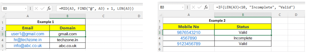
Example 1: Extract Domain Name from Email Address (MID + FIND)

Scenario:

You have a list of emails like "user1@gmail.com" and want to extract just the domain part (gmail.com).

Formula:

=MID(A2, FIND("@", A2) + 1, LEN(A2))

How It Works:

• FIND("@", A2) locates the position of @.
• MID() then extracts everything after the @.

Output:

Email	Domain
user1@gmail.com	gmail.com
hr@techzone.in	techzone.in
info@abc.co.uk	abc.co.uk

---

Example 2: Detect Missing Area Code in Mobile Number (LEN + IF)

Scenario:

You want to check if mobile numbers are missing a country/area code (i.e., fewer than 10 digits).

Formula:

=IF(LEN(A2)<10, "Incomplete", "Valid")

How It Works:

• LEN(A2) checks the number of digits.
• IF() flags numbers shorter than 10 as "Incomplete".

Output:

Mobile No	Status
9876543210	Valid
4567890	Incomplete
9123456789	Valid

---

FAQs – Excel Functions to handle Text

---

Final Thoughts

These 7 Excel text functions give you the power to transform raw data into clean, organized, and useful information. Whether you’re analyzing data, formatting reports, or building dashboards, knowing how to manipulate text will save you time and effort.

What’s Next?

In the next post, we’ll learn about the ROUND Function in Excel