Freeze Panes in Excel

Learn how to use Freeze Panes in Excel to keep headers or important columns always visible while scrolling. Ideal for large data tables.

Have you ever worked with a large Excel sheet and lost track of which row or column you’re on? It can be frustrating to scroll down and not see the headers anymore. That’s where Freeze Panes in Excel comes in!

Freeze Panes is a simple but powerful feature that allows you to lock specific rows or columns in place so they always stay visible as you scroll through your spreadsheet.

In this blog post, you’ll learn:

• What Freeze Panes is and why it’s useful
• How to freeze rows, columns, or both
• The difference between Freeze Top Row, Freeze First Column, and custom Freeze Panes
• Real-life examples using a sales table
• FAQs and bonus tips

---

What is Freeze Panes in Excel?

Freeze Panes is a view setting that allows specific parts of your Excel worksheet to remain visible while the rest of the sheet scrolls.

This is especially helpful when:

• You have long data lists with headers
• You want to compare data across far-right columns
• You want to lock certain fields (like Bill No or Product) in view while analyzing rows

---

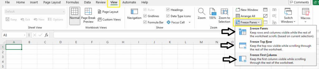
Where to Find Freeze Panes

Go to: View tab → Freeze Panes

You’ll see three main options:

1. Freeze Panes (Custom)
2. Freeze Top Row
3. Freeze First Column

Option 1: Freeze Top Row

Use this when you want to keep the first row (usually headers) visible as you scroll down.

Steps:

• Scroll Up to your Header Row
• Go to the View tab
• Click Freeze Panes > Freeze Top Row

Useful when: Your headers are in Row 1 and you have a long list of data below.

Option 2: Freeze First Column

This keeps Column A always visible as you scroll horizontally.

Steps:

• Scroll Left to your First Column
• Go to the View tab
• Click Freeze Panes > Freeze First Column

Useful when: Column A has critical data like names, IDs, or serial numbers.

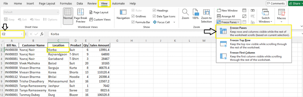
Option 3: Custom Freeze Panes (Rows + Columns)

This is the most flexible option — freeze both rows and columns based on where your cursor is.

Example:

You want to freeze:

• Row 1 (headers)
• Columns A and B (Bill No and Customer Name)

Steps:

1. Click on cell C2 (just below the row and to the right of the columns you want to freeze)
2. Go to View > Freeze Panes > Freeze Panes

Now, Row 1 and Columns A & B will stay locked while the rest scrolls!

---

Read More: Conditional Formatting in Excel and Data Validation in Excel

Real-Life Example: Sales Table

Let’s say your sales table looks like this:

Bill No	Customer Name	Location	Product	Qty	Sales Amount
INV001	Rajeev	Raipur	T-Shirt	5	4500
INV002	Meena	Durg	Hoodie	3	3000
INV003	Ankit	Bilaspur	Kurta	6	5400

You want to scroll down to row 500 while still seeing the headers and customer name.

• Click on C2
• Go to View > Freeze Panes > Freeze Panes
• Now you can scroll vertically and horizontally while always seeing headers and names

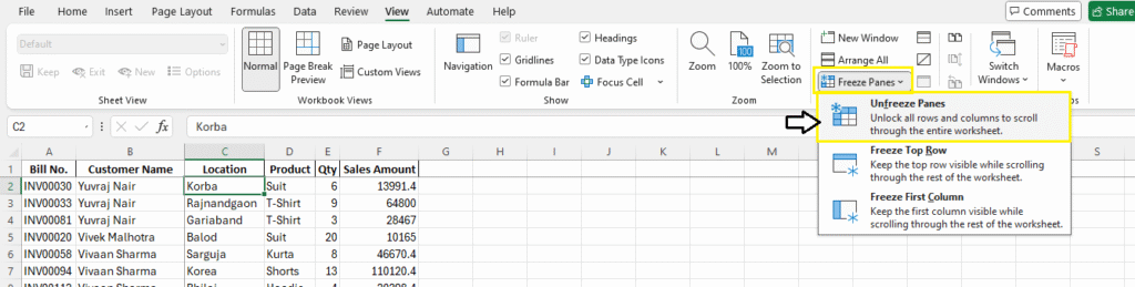
How to Unfreeze Panes

To remove freezing:

• Go to View > Freeze Panes > Unfreeze Panes

This resets the sheet to normal scrolling.

---

Summary

Freeze Panes in Excel is a helpful tool for navigating large spreadsheets. It helps you keep your headers or important columns visible at all times, improving both data entry and analysis.

Use:

• Top Row to keep headers
• First Column for key identifiers
• Custom Freeze Panes for full control

Start using it and stop losing track of your data!

---

Bonus Tips for Using Freeze Panes in Excel

1. Use Freeze Panes with Filters

If you apply filters to your header row (like with Data > Filter Freezing that row helps keep filter options visible while scrolling through large datasets.

Pro Tip: Always freeze the header row before applying filters for better visibility.

2. Freeze Panes with Formulas

If your data includes formulas that reference headers or IDs in frozen columns/rows, keeping them in view can help avoid reference mistakes while editing.

---

3. Combine with Conditional Formatting

Freeze important rows/columns (like targets or customer names), and then use Conditional Formatting to highlight key figures — a great combination for reports and dashboards.

---

4. Use Freeze Panes While Presenting or Sharing

If you plan to share the sheet or present data on a projector/screen, freeze panes to keep context visible for the audience as you scroll.

---

5. Doesn’t Affect Printing

Freeze Panes is a view-only feature. It helps on-screen navigation but does not lock rows/columns on printed pages.

👉 If you want headers to repeat while printing, go to:
Page Layout > Print Titles > Rows to Repeat at Top

---

6. Keyboard Shortcut for Quick Access

There is no direct shortcut, but you can press:

• Alt + W then F then F → to Freeze Panes
• Alt + W then F then U → to Unfreeze Panes

FAQs – Freeze Panes in Excel

What’s Next?

Now that we’ve covered all the basics and intermediate concepts of Excel, let’s move on to Advanced Excel.

In the next post, we’ll learn about the IFS & SWITCH Function in Excel