HLOOKUP in Excel - Tutorials

Learn how to use HLOOKUP in Excel with real-life examples and simple explanations. This beginner-friendly guide will teach you how to perform horizontal lookups to find values across rows instead of columns.

When you’re working with data in Excel, you often need to look up information based on a known value. If your data is organized horizontally (i.e., in rows), then HLOOKUP is the function made for the job.

While many people know about VLOOKUP (Vertical Lookup), fewer are familiar with HLOOKUP — but it’s just as useful when your data is laid out across rows.

In this post, we’ll explain, what is HLOOKUP, how to use it with easy-to-understand examples, and when to use it.

Table of Contents

What is HLOOKUP in Excel?

HLOOKUP stands for Horizontal Lookup. It searches for a value in the first row of a table and returns a value from the same column in a row you specify.

Think of it as looking from left to right across rows, instead of top to bottom.

HLOOKUP Syntax

=HLOOKUP(lookup_value, table_array, row_index_num, [range_lookup])

Let’s break this down:

lookup_value: The value you want to find.
table_array: The data range you want to search in.
row_index_num: The row number (starting from 1) from which to return the value.
[range_lookup]: Optional. Use FALSE for an exact match (recommended), or TRUE for an approximate match.

Example 1: HLOOKUP to Find Student Marks

Let’s say you have student marks stored horizontally:

	A	B	C	D
Subject	Math	English	Science	History
Marks	88	92	79	85

Now, you want to get the mark for Science.

Formula:

=HLOOKUP("Science", A1:E2, 2, 0)

Explanation:

"Science" is the subject you’re looking for.
A1:E2 is your table.
2 tells Excel to return the value from the second row (the Marks).
FALSE ensures you get an exact match.

Result: 79

Use Cases for HLOOKUP

Here are a few examples where HLOOKUP makes your work easier:

Student report cards are stored in a horizontal format.
Monthly sales data where months are column headers.
Survey responses with questions across the top row.
Horizontal data summaries in dashboards or print-ready formats.

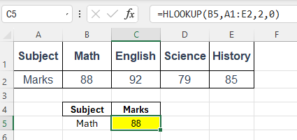
Example 2: HLOOKUP with a Cell Reference

Hlookup in Excel — **HLOOKUP with a Cell Reference**

You can use a cell as the lookup value instead of typing it manually.

If cell B5 contains "Math":

=HLOOKUP(B5,A1:E2,2,0)

Now you can change the subject in B5 and get different results dynamically.

Example 3: HLOOKUP with IFERROR

If the value you’re looking for doesn’t exist, HLOOKUP will return a #N/A error. You can clean this up using IFERROR.

Formula:

=IFERROR(HLOOKUP("Physics", A1:E2, 2, FALSE), "Not Found")

Result: Not Found
This makes your sheet more user-friendly.

HLOOKUP vs VLOOKUP

Feature	HLOOKUP	VLOOKUP
Searches data in	Rows (horizontally)	Columns (vertically)
First search area	First row of the table	First column of the table
Return from	Any row in the same column	Any column in the same row

Choose HLOOKUP when your headings are in the first row and data goes left to right.

Limitations of HLOOKUP

It only searches left to right, not right to left.
You need to count the row index manually.
It’s less flexible than newer functions like XLOOKUP.

If you’re using Excel 365 or Excel 2021, consider switching to XLOOKUP, which combines the best of VLOOKUP, HLOOKUP, and more.

Quick Summary

HLOOKUP is used when your data is laid out in rows, not columns.
Great for student marks, monthly summaries, and survey results.
Syntax: =HLOOKUP(lookup_value, table_array, row_index_num, FALSE)
Combine it with IFERROR for cleaner results.

Final Thoughts

While HLOOKUP in Excel may not be as popular as VLOOKUP, it’s still very useful when your data is organized horizontally. For small reports, summaries, or education-related work, this function can be a real time-saver.

Try it out today—flip your tables and let HLOOKUP do the work!

What’s Next?

In the next post, we’ll learn about the INDIRECT Function in Excel

Spread the love