|
Getting your Trinity Audio player ready...
|
Why Learn Index and Match in Excel?
When most beginners learn Excel lookup functions, they start with VLOOKUP. It’s useful but comes with many limitations. As your Excel skills grow, you’ll find that INDEX and MATCH offer a more powerful, more flexible, and more accurate way to look up values.
If you’re serious about Excel (for data entry, reports, HR, finance, MIS, etc.), understanding INDEX and MATCH in Excel is a must.
What is INDEX in Excel?
The INDEX Function returns the value from a specific cell in a range based on the row and column numbers you provide.
Syntax:
=INDEX(array, row_num, [column_num])
- array: The data range.
- row_num: The row number to return data from.
- column_num: (Optional) If it’s a 2D table, specify the column.
Example:
You have a list of items:
| A | B |
|---|---|
| Apple | 50 |
| Banana | 30 |
| Mango | 40 |
=INDEX(B2:B4, 2)
👉 Result: 30 (returns the value from the 2nd row in the range)
What is MATCH in Excel?
The MATCH Function returns the position of a value in a row or column.
Syntax:
=MATCH(lookup_value, lookup_array, [match_type])
- lookup_value: What you’re searching for.
- lookup_array: Where you’re searching.
- match_type: Use
0for an exact match.
Example:
You want to find the position of “Mango”:
=MATCH("Mango", A2:A4, 0)
👉 Result: 3 (because Mango is the 3rd item)
How INDEX and MATCH in Excel Work Together
When you combine both, you can do something very powerful:
- Use
MATCHto find the row number - Use
INDEXto return the value at that row
Combined Formula:
=INDEX(B2:B4, MATCH("Mango", A2:A4, 0))
Explanation:
MATCH("Mango", A2:A4, 0)returns3INDEX(B2:B4, 3)returns40
👉 Final Result: 40 (The price of Mango)
Why INDEX and MATCH in Excel Is Better Than VLOOKUP
| Feature | INDEX & MATCH | VLOOKUP |
|---|---|---|
| Looks left or right | ✅ Yes | ❌ No (only right) |
| Works if columns change | ✅ Yes | ❌ Breaks if column moves |
| More flexible | ✅ Yes | ⚠️ Limited |
| Faster with big data | ✅ Yes | ❌ Slower |
| Supports dynamic arrays | ✅ Yes (with Excel 365) | ❌ No |
Real-Life Examples
Example 1: Get Product Price
| A | B |
|---|---|
| Product | Price |
| Pen | 10 |
| Pencil | 5 |
| Eraser | 3 |
Formula:
=INDEX(B2:B4, MATCH("Pencil", A2:A4, 0))
Result: 5
Example 2: Get Employee Department
| A | B |
|---|---|
| Name | Department |
| Ramesh | HR |
| Suresh | IT |
| Kamal | Finance |
Lookup Kamal’s department:
=INDEX(B2:B4, MATCH("Kamal", A2:A4, 0))
👉 Result: Finance
Example 3: Two-Way Lookup (Row + Column Match)
| A | B | C |
|---|---|---|
| Name | Maths | English |
| Ravi | 88 | 75 |
| Anjali | 90 | 85 |
| Neha | 70 | 92 |
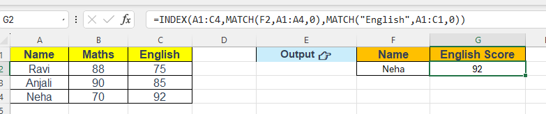
You want to find Neha’s English score.
Formula:
=INDEX(A1:C4, MATCH("Neha", A1:A4, 0), MATCH("English", A1:C1, 0))
👉 Result: 92
Example 4: Using INDEX with OFFSET to Get a Dynamic Value
Scenario:
You want to get the first product name from a dynamic range that starts from a specific cell (e.g., B2), and covers a number of rows and columns that may change based on a formula.
Product Table (A1:C4):
| A | B | C |
|---|---|---|
| Product | Price | Stock |
| Mouse | 400 | 100 |
| Keyboard | 700 | 50 |
| Monitor | 6000 | 30 |
Goal:
Use OFFSET to define the range starting from A1 with 3 rows and 1 column (i.e., the Product list), and use INDEX to get the first product name from that range.
Formula:
=INDEX(OFFSET(A1,1,0,3,1),1)
Explanation:
OFFSET(A1,1,0,3,1)
→ Starts 1 row below A1, stays in the same column, and returns a range of 3 rows × 1 column:
This refers to the rangeA2:A4(Mouse,Keyboard,Monitor).INDEX(...,1)
→ Returns the first value from the rangeA2:A4, which isMouse.
Result: Mouse
Example 5: Get Max QTY Using INDEX + OFFSET + MAX + COUNTA
Scenario:
You have a sales table where each customer has QTY and VAL columns for each year (e.g., 2022 QTY, 2022 VAL, 2023 QTY, 2023 VAL, etc.). The number of years may grow or shrink.
Sample Table:
| A | B | C | D | E | F | G |
|---|---|---|---|---|---|---|
| Customer | 2022 QTY | 2022 VAL | 2023 QTY | 2023 VAL | 2024 QTY | 2024 VAL |
| A | 100 | 5000 | 130 | 7000 | 90 | 4500 |
| B | 80 | 4000 | 120 | 7200 | 110 | 6000 |
Goal:
Get the maximum QTY sold to Customer A, regardless of how many years are included.
Formula Using COUNTA:
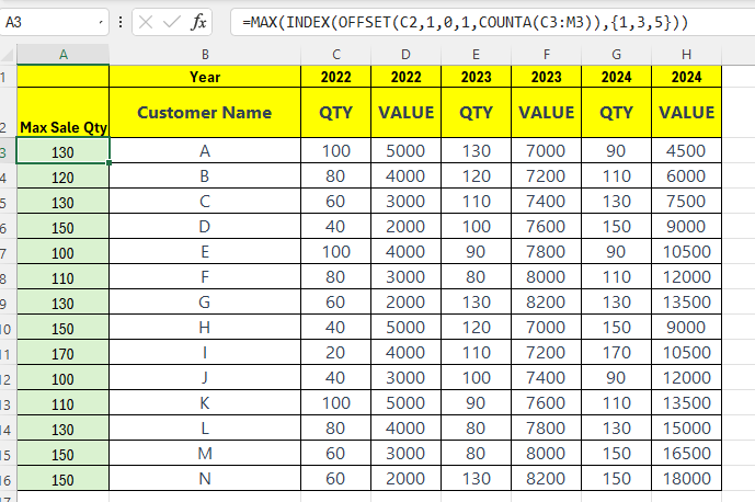
=MAX(INDEX(OFFSET(B3, 0, 0, 1, COUNTA(B2:Z2)), {1,3,5}))
Explanation:
OFFSET(B3, 0, 0, 1, COUNTA(B2:Z2))- Starts from B3 (the first year QTY cell)
- Goes down 1 row and across
COUNTA(B2:Z2)columns (number of filled year-related columns from the header row) - Returns a dynamic row range like
B3:G3, depending on how many year columns exist
INDEX(..., {1,3,5})- Picks every odd-numbered column from the result (i.e., 1st, 3rd, 5th QTY columns)
- Skips the VAL columns (which are 2nd, 4th, etc.)
MAX(...)- Returns the maximum quantity among the QTY columns
Final Output for Customer A:
- QTYs = 100 (2022), 130 (2023), 90 (2024)
👉 Result:130
Why This Works with COUNTA
COUNTA(B2:Z2)counts how many header columns are filled — ensures your range is always correct, even if you add 2025, 2026, etc.- Works whether you have 2 years or 10 — no need to change the formula!
When to Use This Combo:
- When your data range changes dynamically based on filters or formulas.
- To create advanced reports that adjust lookup areas automatically.
- In dashboards, starting points and lengths are controlled by user inputs.
Also Read: Excel COUNT & COUNTA Functions and Excel MIN & MAX Functions
Download Practice File:
Common Errors and Fixes
| Error | Reason | Fix |
|---|---|---|
#N/A | No exact match found | Check for spelling or extra spaces |
#REF! | Row/column number out of range | Verify your array size |
#VALUE! | Wrong data types used | Ensure correct input in MATCH/INDEX |
Also Read: IFERROR & IFNA in Excel
Pro Tips for Beginners
- Always use
0in MATCH for exact matches. - Use named ranges for better readability.
- Combine with
IFERRORfor cleaner output:
=IFERROR(INDEX(B2:B4, MATCH("Pencil", A2:A4, 0)), "Not Found")
- Try using Data Validation dropdowns to make dynamic lookups.
Summary
INDEXgives a value at a specific position.MATCHfinds the position of a value.- Combined together, they offer a powerful alternative to VLOOKUP.
- They are more flexible, faster, and less prone to errors.
Also Read: VLOOKUP in Excel and HLOOKUP in Excel
Mastering
INDEX and MATCHin Excel will take your Excel skills to the next level!
FAQs – Index and Match in Excel
What does MATCH return?
It returns the position (row or column number) of the value you’re searching for.
Can INDEX and MATCH be used with two-way lookup?
Yes, you can nest two MATCH functions for rows and columns to create a 2D lookup.
Is INDEX-MATCH faster than VLOOKUP?
Yes, especially when working with large datasets.
Final Words
Learning Index and Match in Excel is one of the most valuable upgrades you can give to your spreadsheet skills. It unlocks flexibility, precision, and efficiency that every Excel user will appreciate.
Whether you’re in accounting, education, HR, marketing, or MIS—start using INDEX and MATCH today, and you’ll never go back to VLOOKUP.
What’s Next?
In the next post, we’ll learn about the Pivot Table in Excel