Offset Function in Excel

What is the OFFSET Function in Excel?

The OFFSET function in Excel returns a cell or range of cells that is a specified number of rows and columns away from a starting point (reference). It’s especially powerful for dynamic range creation, data analysis, and flexible lookups.

If you want to build formulas that automatically adjust when your data grows or shifts, then OFFSET is a function you must learn.

---

OFFSET Function Syntax

=OFFSET(reference, rows, cols, [height], [width])

Argument Details:

Argument	Description
reference	The starting cell or range.
rows	How many rows to move up/down.
cols	How many columns to move left/right.
height (optional)	Number of rows in the returned range.
width (optional)	Number of columns in the returned range.

---

Basic Example of OFFSET

Scenario:

You have sales data in B2:B6. You want to get the value 3 rows below B2 (i.e., B5).

Formula:

=OFFSET(B2, 3, 0)

👉 Result: Value in B5

---

Real-Life Examples of OFFSET Function in Excel

Example 1: Get Cell Value Dynamically

Suppose your starting cell is A1, and you want the value 2 rows down and 1 column to the right (i.e., cell B3).

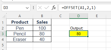
=OFFSET(A1, 2, 1)

This returns the value of B3.

---

Example 2: Create a Dynamic Range

If your data grows every day, and you want to always calculate the average of the latest 5 entries (means average of the last 5 entries), use:

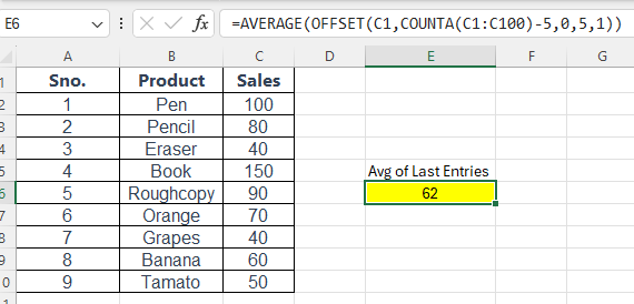
=AVERAGE(OFFSET(C1,COUNTA(C1:C100)-5,0,5,1))

• COUNTA counts how many values are present
• OFFSET creates a range 5 rows tall, ending at the last entry
• AVERAGE calculates the average of those 5 values

Pro Tips: Great for dashboards or rolling averages!

👉 Practice File: Click me to get Practice File

Also Read: Excel AVERAGE Function and Excel COUNT & COUNTA Functions

Example 3: Create a Dynamic Filter Range with OFFSET + COUNTA

Scenario:

You have a growing list of customer names in column A starting from cell A2. You want to create a dynamic named range or a data validation dropdown that automatically includes all entries — no need to manually update the range when new names are added.

---

Sample Data (A2:A6):

A
Ramesh
Suresh
Kamal
Neha
Jaya

If you add more names below, the filter/dropdown should pick them automatically.

---

Formula:

=OFFSET(A2, 0, 0, COUNTA(A2:A100), 1)

---

Explanation:

• A2 → Starting reference (first data cell)
• 0, 0 → No row or column shift
• COUNTA(A2:A100) → Counts how many non-empty rows exist (customer names)
• 1 → Width of 1 column

Note: This formula returns a range from A2 down to the last non-empty cell, based on the number of filled cells.

---

How to Use This in Excel:

1. Create a Dynamic Named Range

• Go to Formulas → Name Manager → New
• Name: CustomerList
• Refers to: =OFFSET(Sheet1!$A$2, 0, 0, COUNTA(Sheet1!$A$2:$A$100), 1)

2. Use in Data Validation

• Select a cell where you want the dropdown
• Go to Data → Data Validation
• Choose List
• In the Source box, enter: =CustomerList

Now, as you add or remove names in column A, the dropdown list will automatically update.

Example 4: Create a Dependent Dropdown in Excel Using OFFSET

Let’s say:

• Dropdown 1 (Category): Select a product type like Fruits, Vegetables, or Beverages
• Dropdown 2 (Subcategory): Automatically lists items based on selected category

---

Step-by-Step Example

Step 1: Prepare Your Data

Sheet1 – Named DropdownData

A	B	C
Fruits	Vegetables	Beverages
Apple	Carrot	Tea
Banana	Tomato	Coffee
Mango	Potato	Juice

---

Step 2: Create Dynamic Named Ranges Using OFFSET + COUNTA

Go to Formulas → Name Manager → New, and define:

Name: Fruits

=OFFSET(DropdownData!$A$2, 0, 0, COUNTA(DropdownData!$A$2:$A$100), 1)

Name: Vegetables

=OFFSET(DropdownData!$B$2, 0, 0, COUNTA(DropdownData!$B$2:$B$100), 1)

Name: Beverages

=OFFSET(DropdownData!$C$2, 0, 0, COUNTA(DropdownData!$C$2:$C$100), 1)

These ranges will auto-expand as you add more items under each category.

---

Step 3: Create Category Dropdown (Main Dropdown)

On another sheet (e.g., Sheet2):

1. Select a cell (e.g., A2)
2. Go to Data → Data Validation
3. Choose List, and set source to: CopyEditFruits,Vegetables,Beverages

Now, you can select a category.

---

Step 4: Create Dependent Dropdown (Subcategory)

1. Select cell B2 (next to the category dropdown)
2. Go to Data → Data Validation
3. Choose List, and in Source, use: =INDIRECT(A2)

👉 This uses the selected category in A2 as the name of the range (like =Fruits, =Vegetables, etc.), pulling the correct list using INDIRECT.

---

Example in Action:

A (Category)	B (Subcategory)
Fruits	Apple
Vegetables	Carrot
Beverages	Tea

As soon as you change A2, the subcategory list in B2 updates accordingly!

---

Important Tips:

• Make sure your category names match the named ranges exactly (case-insensitive, but no spaces or special characters unless handled).
• Avoid merging cells in your source table.
• You can hide the DropdownData sheet to keep your workbook clean.

OFFSET Function Is Volatile

OFFSET is a volatile function, meaning:

• It recalculates every time anything in the worksheet changes
• Can slow down performance in large files

Tips: Use with care in large data models!

---

Common Use Cases of OFFSET Function in Excel

• Creating dynamic charts
• Automating rolling averages
• Extracting dynamic rows/columns
• Building pivot-compatible dynamic ranges
• Flexible dashboard inputs

Summary

The OFFSET function in Excel lets you dynamically reference a cell or range that is a certain number of rows and columns away from a starting point. It’s perfect for:

• Creating flexible and dynamic data ranges
• Building smarter reports and dashboards
• Automating lookup behavior based on position

With OFFSET + COUNTA and INDIRECT, you can build fully dynamic, expandable, and dependent dropdown lists in Excel. Perfect for:

• Product category + item selection
• Country + state + city selection
• Department + employee dropdowns

However, since it’s volatile, use it wisely in large files.

FAQs About OFFSET Function in Excel

What’s Next?

In the next post, we’ll learn about the Excel Functions to Handle Text