Pivot Table in Excel

Master Pivot Table in Excel from basic to advanced. Learn how to summarize, analyze, and visualize data effectively using real-world examples.

---

If you work with large amounts of data in Excel, manually analyzing it can be time-consuming and error-prone. This is where Pivot Tables come in. With just a few clicks, Pivot Tables help you summarize and analyze data efficiently.

Whether you’re a beginner or looking to level up your skills, this guide will teach you how to use Pivot Tables from basic to advanced – with step-by-step instructions, real-life sales examples.

What is a Pivot Table?

A Pivot Table is a tool in Excel that allows you to:

• Summarize large datasets
• Group and filter data dynamically
• Calculate totals, averages, percentages, and more

It’s one of the most powerful features in Excel for reporting and decision-making.

---

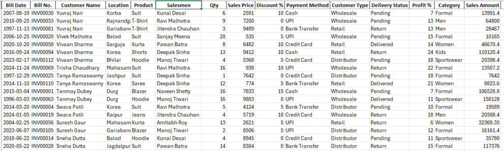
Sample Dataset Used in This Guide

---

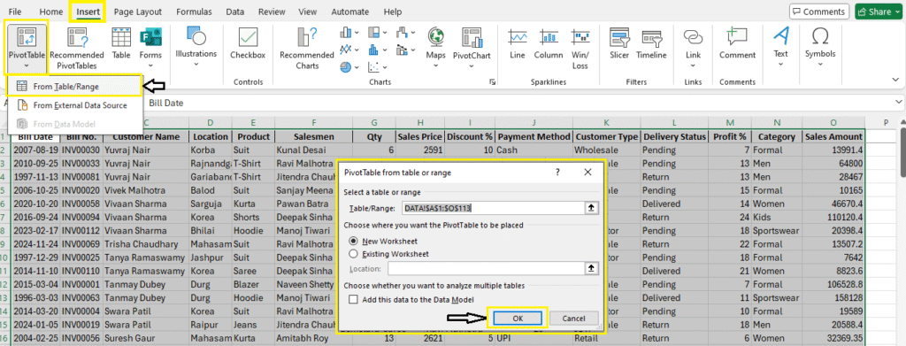
How to Insert a Pivot Table

1. Select your data range (e.g., A1:F113)
2. Go to the Insert tab
3. Click PivotTable or (use shortcut: Alt+N+V then press Enter Key)
4. Choose whether to place it in a New Worksheet or an Existing Worksheet
5. Click OK

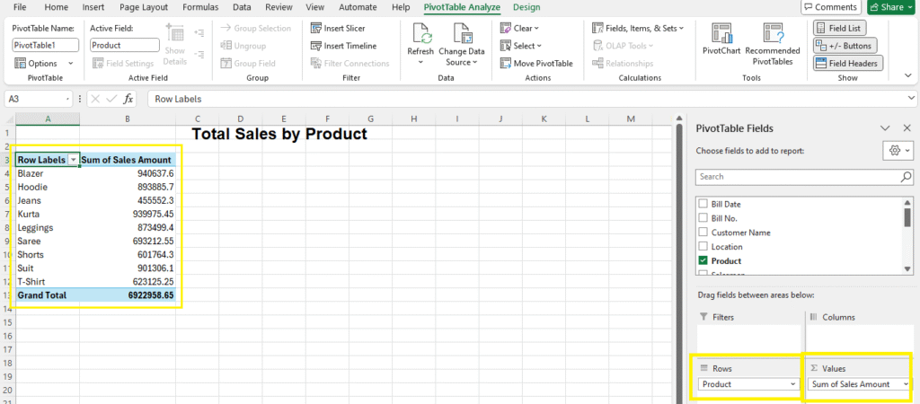
Example 1: Total Sales by Product

Steps:

1. Drag Product to Rows
2. Drag Sales Amount to Values

Result:

Product	Sum of Sales Amount
Blazer	940637.6
Hoodie	893885.7
Jeans	455552.3
Kurta	939975.45

---

Read More: VLOOKUP in Excel and SUMIF & SUMIFS in Excel

Grouping Data: Group by Location or Customer

Example 2: Total Sales by Location with Filter

• Drag Location to Rows
• Drag Sales Amount to Values

Filter data in Pivot Table:

Filters are used to select what data you see.
In this example, there are two filters enabled: Salesmen and Delivery Status.

The filters are set to:
Salesmen = Naveen Shetty and
Delivery Status = Delivered.

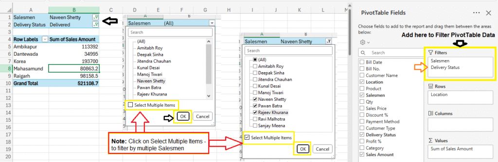
Note: Click on Select Multiple Items – to filter by multiple Salesmen

---

Example 3: Total Sales by Customer

• Drag Customer Name to Rows
• Drag Sales Amount to Values

---

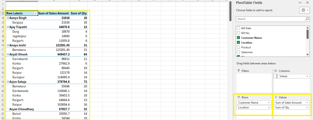
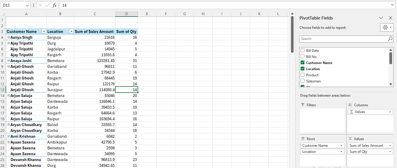
Example 4: Total Sales Amount and Qty by Customer and Location

Steps:

1. Drag Customer and Location to Rows
2. Sales Amount and Qty to Values

Now Your Table will look like this:

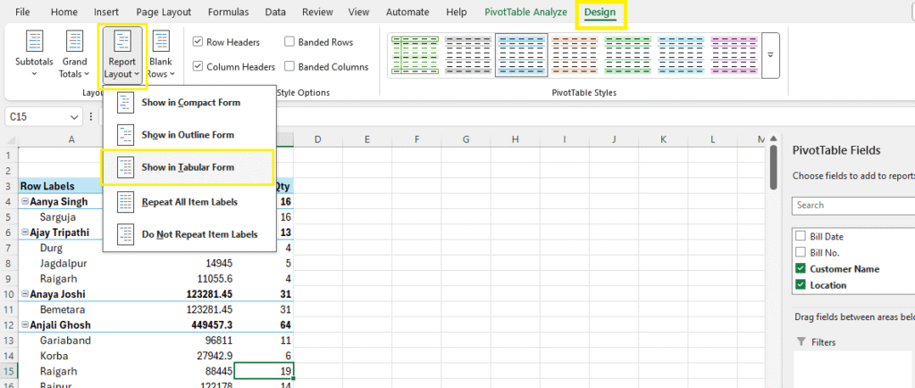
Step 2: Let’s convert this data to Tabular Form, meaning:

• Customer Name in Column A,
• Location in Column B
• Sales Amount in Column C and Qty in Column D
• Click anywhere in Pivot Table and go to Design Tab, then follow bellow steps:

Step 1: Design Tab > Report Labout > Show in Tabular Form

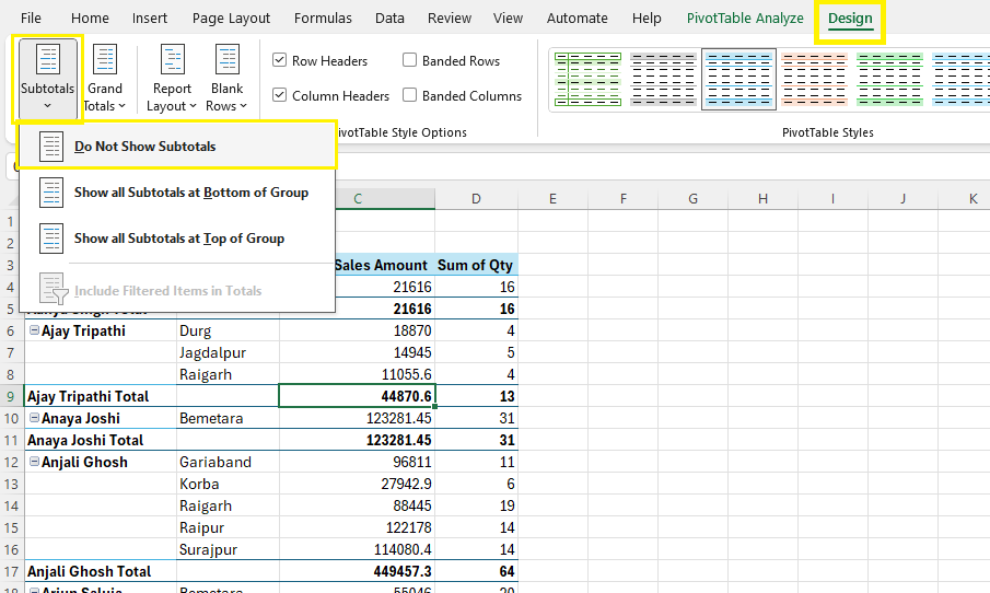
Step 2: Design Tab > Subtotals > Do Not Show Subtotals

Step 3: Design Tab > Report Layout > Repeat All Item Labels

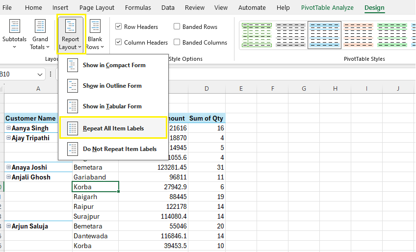
Final Output:

---

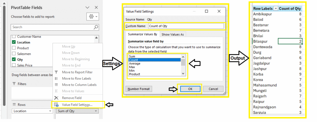
Custom Calculations in Pivot Table

You can add:

• Count instead of sum
• Averages
• Max, Min

Steps:

• Click the dropdown in Values → Value Field Settings
• Choose Average, Count, etc.

---

Advanced Pivot Table Techniques

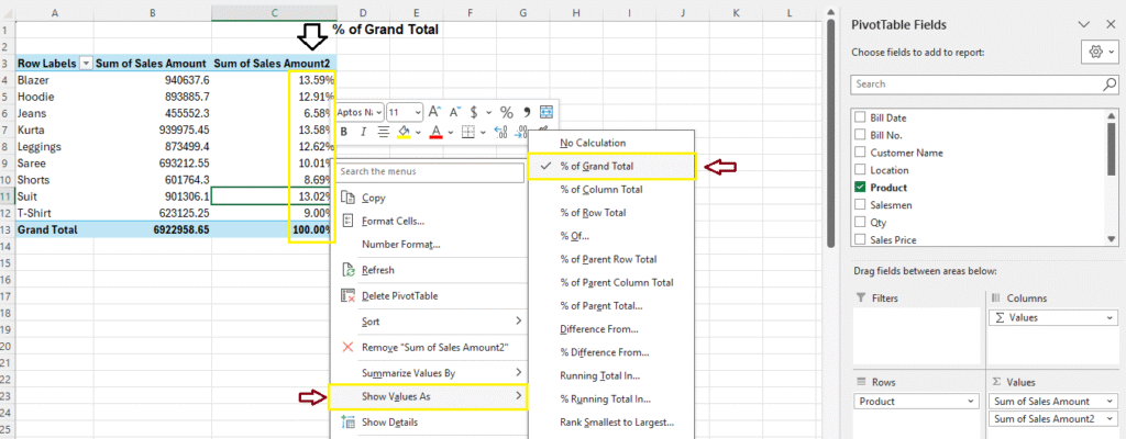
1. Show % of Total Sales – Contribution of Each Row in 100%

Show how much each product contributes to total sales.

• Right-click Sales Amount field
• Choose Show Values As > % of Grand Total

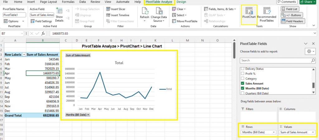
2. Create Pivot Charts

Go to PivotTable Analyze > PivotChart

• Create Bar, Column, Pie, etc.

Note: We will learn all about Charts & Pivot Charts in a separate tutorial.

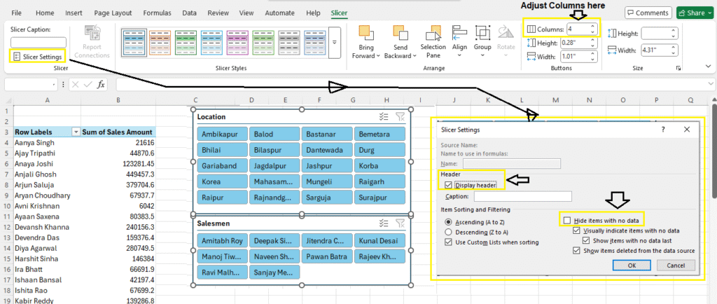
3. Use Slicers to Filter Pivot Tables

Slicers are visual filters.

• Go to Insert > Slicer
• Select fields like Location or Product

Note: Slicers in Pivot Tables are used to filter data quickly and easily with clickable buttons visually.

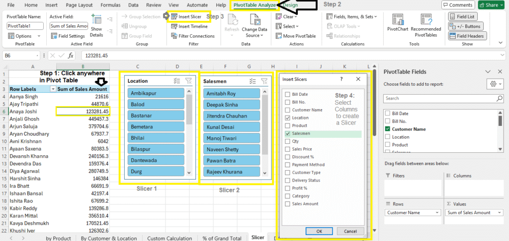
Note: Click on Slicer to Change it’s Settings (under Slicer Tab)

4. Add Multiple Value Fields

You can drag Qty and Sales Amount to Values to show both.

Note: For Practice

---

Real-Life Example Scenarios

Example 1: Compare Sales by Location

• Rows: Location
• Values: Sales Amount

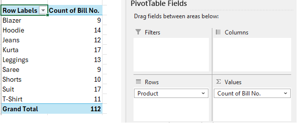
Example 2: Count of Orders by Product

• Rows: Product
• Values: Bill No (set to Count)

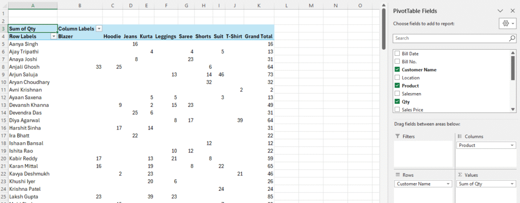
Example 3: Customer Purchase Summary

• Rows: Customer Name
• Columns: Product
• Values: Qty

Example 4: Monthly Sales Trend

• Rows: Month (from Bill Date)
• Values: Sales Amount
• Show as Line Chart

---

Refresh Pivot Table (when Source Data Changes)

• When your source data changes, right-click the Pivot Table → Refresh
• To update automatically: Go to PivotTable Options > Data > Refresh data when opening file

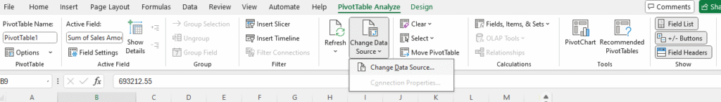
Change Data Source

Change Data Source lets you update the range of your Pivot Table when your original data grows or changes.

• Click on your Pivot Table
• PivotTable Analyze Tab > Change Data Source
• Select Data Range > OK

---

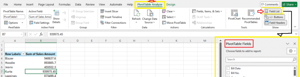
Hide/Unhide PivotTable Fields – Field List

---

Tips & Troubleshooting

• Always format source data as a Table before creating a Pivot
• Remove blank rows for accurate calculations
• Check for duplicates in headers

Download Practice Material

---

Summary

Pivot Tables are one of Excel’s best features for summarizing and analyzing data. From simple totals to advanced comparisons and filters, they save time and make reports dynamic.

Whether you’re managing sales, projects, or MIS reporting, Pivot Tables should be in your skillset.

FAQs – Pivot Table in Excel

---

Final Thoughts

Pivot Tables are not just for analysts — anyone working with Excel can use them to gain insights quickly. Start with basic summaries, and as your confidence grows, try out slicers, charts, and advanced calculations.

What’s Next?

In the next post, we’ll learn about the Error Handling in Excel