Subtotal and Aggregate Function in Excel

Learn how to use SUBTOTAL and AGGREGATE function in Excel to summarize data efficiently, with simple examples and expert tips for beginners.

When dealing with large data in Excel, it’s important to calculate subtotals, ignore hidden rows, and apply multiple types of summaries like average, count, max, or sum. Thankfully, Excel provides two very handy functions for this purpose:

• SUBTOTAL()
• AGGREGATE()

These functions are more flexible than standard formulas like SUM() or AVERAGE(), especially when working with filtered or hidden data. In this blog post, you’ll learn how each function works, when to use them, and how they can improve your productivity in Excel.

---

What is the SUBTOTAL Function in Excel?

Syntax:

=SUBTOTAL(function_num, ref1, [ref2], …)

• function_num: A number (1–11 or 101–111) that specifies the summary operation (e.g., SUM, AVERAGE, etc.)
• ref1, ref2, etc.: Ranges to include

All SUBTOTAL Function Numbers:

function_num	Summary Function	Hidden Rows Ignored	Description
1	AVERAGE	❌	Average including manually hidden rows
2	COUNT	❌	Count numbers in all rows
3	COUNTA	❌	Count non-blank cells
4	MAX	❌	Maximum value
5	MIN	❌	Minimum value
6	PRODUCT	❌	Product of values
7	STDEV	❌	Sample standard deviation
8	STDEVP	❌	Population standard deviation
9	SUM	❌	Sum includes manually hidden rows
10	VAR	❌	Sample variance
11	VARP	❌	Population variance
101–111	Same functions	✅	Ignores manually hidden and filtered rows

Hidden Row Behavior Clarified

Code Type	Filtered Rows	Manually Hidden Rows
1–11	Ignored	Included
101–111	Ignored	Ignored

Conclusion:

• Both sets ignore filtered-out rows.
• Only 101–111 ignore manually hidden rows as well.

Example 1: Subtotal of Visible Sales

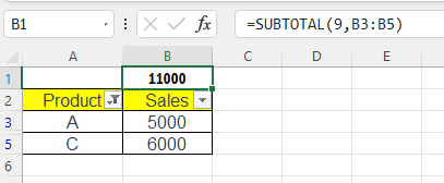
Product	Sales
A	5000
B	7000
C	6000

If rows are filtered, this formula will only total visible ones:

=SUBTOTAL(109, B2:B4)

Result: Sum of only visible sales

---

What is the AGGREGATE Function in Excel?

The AGGREGATE() function goes beyond SUBTOTAL() by allowing:

• More functions (like LARGE, SMALL, MEDIAN)
• More control over ignoring errors, hidden rows, and nested SUBTOTAL/AGGREGATE functions

Syntax:

=AGGREGATE(function_num, options, ref1, [ref2], …)

• function_num: Same concept as SUBTOTAL, with extended options
• options: Controls what to ignore (errors, hidden rows, etc.)
• ref1: The range

All AGGREGATE Function Numbers:

Function Number	Summary Function
1	AVERAGE
2	COUNT
3	COUNTA
4	MAX
5	MIN
6	PRODUCT
7	STDEV.S
8	STDEV.P
9	SUM
10	VAR.S
11	VAR.P
12	MEDIAN
13	MODE.SNGL
14	LARGE
15	SMALL
16	PERCENTILE.INC
17	QUARTILE.INC
18	PERCENTILE.EXC
19	QUARTILE.EXC

AGGREGATE Options Explained:

Option Number	What It Ignores	Description
0	Nothing	Includes hidden rows and errors
1	Hidden rows	Ignores manually hidden rows
2	Error values	Ignores #DIV/0!, #N/A, etc.
3	Hidden rows & error values	Best for clean summary of visible good data
4	Nested SUBTOTAL/AGGREGATE functions	Ignores nested subtotals
5	Hidden rows + nested SUBTOTAL/AGGREGATE	Useful in filtered nested reports
6	Errors + nested SUBTOTAL/AGGREGATE	For error-prone data + subtotals
7	Hidden rows + errors + nested functions	Full ignore mode for cleanest output

Example 2: Ignore Errors While Taking Average

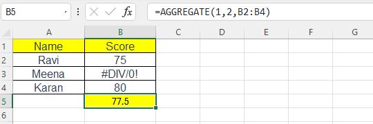
Name	Score
Ravi	75
Meena	#DIV/0!
Karan	80

=AGGREGATE(1, 2, B2:B4)

Result: Average of 75 and 80 (ignores the error)

---

SUBTOTAL vs AGGREGATE: Key Differences

Feature	SUBTOTAL	AGGREGATE
Filters Aware	✅	✅
Ignores Hidden Rows	Only with 101–111	✅ With option 1+
Supports Errors	❌	✅
More Functions	❌ (limited)	✅ (19 total)
Complex Ranges	❌	✅
Nested Support	❌	✅

---

Real-Life Use Cases

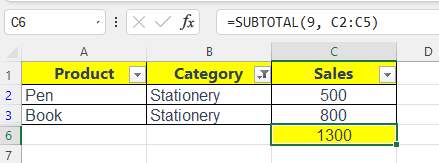
Example 3: Subtotal of Sales in a Filtered Table

Imagine you’re managing a small shop and have this sales data:

Product	Category	Sales
Pen	Stationery	500
Book	Stationery	800
T-Shirt	Apparel	1500
Jeans	Apparel	2000

Now, suppose you filter the table to show only “Stationery” items (like Pen & Book).

If you use:

=SUBTOTAL(9, C2:C5)

This will sum only the visible rows (in this case, Pen and Book).

• 9 stands for SUM
• SUBTOTAL automatically ignores filtered-out rows

Result:

500 + 800 = 1300

Note: If you use SUBTOTAL(109, ...) and manually hide rows (not just filter), it will also ignore those manually hidden rows.

Example 4: Find 2nd Largest Visible Value

Sales

5000

7000

6500

=AGGREGATE(14, 1, B2:B4, 2)

Result: 6500 (2nd largest sales number ignoring hidden rows)

---

Tips and Best Practices

• Use SUBTOTAL(109, range) for summing filtered data and hidden rows
• Use SUBTOTAL(9, range) if hidden rows should still be included
• Use AGGREGATE(1, 2, range) to ignore errors when averaging
• Always match function_num correctly to what you want
• Use AGGREGATE when your dataset might include errors

Download Practice File

---

Summary

SUBTOTAL and AGGREGATE Function in Excel are game-changers when analyzing filtered data, skipping errors, or needing flexible summaries. While SUBTOTAL is easier and perfect for filtered lists, AGGREGATE is more powerful and handles complex data scenarios.

Whether you’re a beginner or working on professional reports, mastering these functions will make your Excel work smarter and faster.

Also Read: Excel SUM Function

---

FAQs – Subtotal and Aggregate Function in Excel

What’s Next?

In the next post, we’ll learn about the Conditional Formatting in Excel