|
Getting your Trinity Audio player ready...
|
When you start working with large sets of data in Excel, one of the most useful tools you can learn is VLOOKUP. It’s a function that helps you search for values in your spreadsheet—almost like looking up a word in a dictionary.
Let’s break it down into easy steps, with examples, use cases, and tips—perfect for beginners!
What is VLOOKUP in Excel?
VLOOKUP stands for Vertical Lookup. It’s used to search for a value in the first column of a range and return a value in the same row from another column.
In simple words:
“If you know what to look for, VLOOKUP helps you find related data in a table.”
VLOOKUP Syntax
Here’s the structure of the VLOOKUP formula:
=VLOOKUP(lookup_value, table_array, col_index_num, [range_lookup])
Let’s understand each part:
- lookup_value: The value you want to search for (e.g., a product name).
- table_array: The range of cells that contains the data (e.g., A2:D100).
- col_index_num: The column number in the range from which to return the value.
- range_lookup: Optional. Use FALSE for an exact match (recommended). Use TRUE for an approximate match.
Example 1: VLOOKUP to Find Product Price
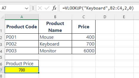
Imagine you have a product list:
| Product Code | Product Name | Price |
|---|---|---|
| P001 | Mouse | 400 |
| P002 | Keyboard | 700 |
| P003 | Monitor | 6000 |
Now, you want to find the price of “Keyboard”.
Formula:
=VLOOKUP("Keyboard", B2:C4, 2, 0)
Explanation:
"Keyboard"is what you are looking for.B2:C4is the data range.- 2 is the column number of the price.
- 0 or
FALSEmeans you want an exact match.
Result: 700
Example 2: VLOOKUP Using a Cell as Lookup Value
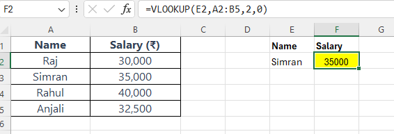
Scenario:
You’re calculating the salary of an employee by selecting their name from a dropdown list.
Data Table (A2:B5):
| A | B |
|---|---|
| Name | Salary (₹) |
| Raj | 30,000 |
| Simran | 35,000 |
| Rahul | 40,000 |
| Anjali | 32,500 |
Lookup Cell:
Suppose in cell E2, you type or select the name Simran.
Formula:
=VLOOKUP(E2, A2:B5, 2, 0)
Result: 35,000
Example 3: VLOOKUP from a Different Sheet
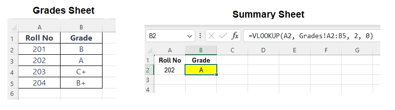
Scenario:
You have a summary sheet and a grades sheet in the same workbook. You want to fetch a student’s grade from the Grades sheet.
On Sheet “Grades” (A2:B5):
| A | B |
|---|---|
| Roll No | Grade |
| 201 | B |
| 202 | A |
| 203 | C+ |
| 204 | B+ |
On Sheet “Summary”:
In cell A2, you enter the roll number 202.
Formula (in Summary sheet):
=VLOOKUP(A2, Grades!A2:B5, 2, 0)
Result: A
Example 4: VLOOKUP from a Different Workbook
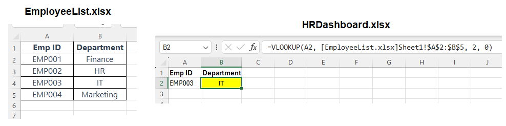
Scenario:
You maintain employee details in one file (EmployeeList.xlsx) and want to fetch an employee’s department in another workbook (HRDashboard.xlsx).
In EmployeeList.xlsx (Sheet1, A2:B5):
| A | B |
|---|---|
| Emp ID | Department |
| EMP001 | Finance |
| EMP002 | HR |
| EMP003 | IT |
| EMP004 | Marketing |
In HRDashboard.xlsx, you type EMP003 in cell A2.
Formula (while both files are open):
=VLOOKUP(A2, '[EmployeeList.xlsx]Sheet1'!$A$2:$B$5, 2, 0)
Result: IT
⚠️ When the source file is closed, Excel will display the full file path:
=VLOOKUP(A2, 'C:\Users\YourName\Documents\[EmployeeList.xlsx]Sheet1'!$A$2:$B$5, 2, 0)
Example 5: VLOOKUP with IFERROR to Handle Missing Values
Scenario:
You’re trying to get product prices, but sometimes the product name entered doesn’t exist in your list.
Product Table (A2:B4):
| A | B |
|---|---|
| Charger | 500 |
| Power Bank | 1500 |
| Cable | 250 |
You enter “Headphones” in D2, which doesn’t exist.
Formula:
=IFERROR(VLOOKUP(D2, A2:B4, 2, 0), "Not Found")
Result: Not Found
Instead of showing #N/A, it shows a clean message.
Example 6: VLOOKUP with Column Index Array to Get Multiple Values
Scenario:
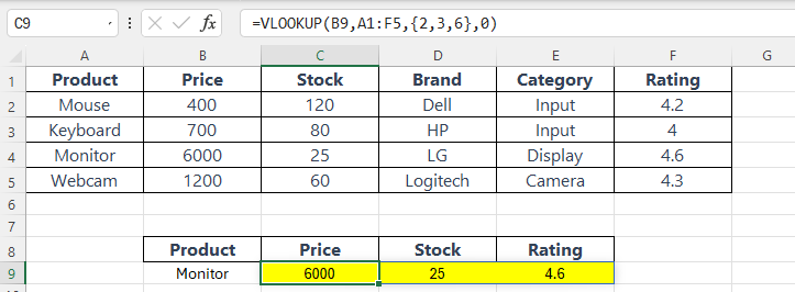
You want to retrieve multiple details (such as price, stock, and rating) for a single product using a single VLOOKUP formula.
Product Table (A1:F5):
| A | B | C | D | E | F |
|---|---|---|---|---|---|
| Product | Price | Stock | Brand | Category | Rating |
| Mouse | 400 | 120 | Dell | Input | 4.2 |
| Keyboard | 700 | 80 | HP | Input | 4.0 |
| Monitor | 6000 | 25 | LG | Display | 4.6 |
| Webcam | 1200 | 60 | Logitech | Camera | 4.3 |
👉 Goal:
Look up “Monitor” and return Price, Stock, and Rating using one formula.
Step-by-Step
Lookup Value in B9:
Monitor
Formula in C9 (and it spills into D9 & E9):
=VLOOKUP(B9,A1:F5,{2,3,6},0)
Result:
| B | C | D | E |
|---|---|---|---|
| Monitor | 6000 | 25 | 4.6 |
{2,3,6}tells Excel to return the 2nd, 3rd, and 6th columns from the lookup table.- This formula automatically spills across the row into 3 cells.
⚠️ Requirements:
- ✅ Excel 365 or Excel 2021+ (for dynamic array support).
- ❌ Will not work in Excel 2016 or older—it will return only one result or give an error.
Combine with IFNA (Optional):
To handle errors (like missing product):
=IFNA(VLOOKUP(B9,A1:F5,{2,3,6},0), "Not Found")
This will return "Not Found" in each column if the product is missing.
👉 Also Read: IFERROR & IFNA in Excel
Use Cases:
- Retrieve multiple attributes (price, quantity, brand) at once.
- Build product cards, dashboards, or summary reports.
- Great for customer, product, or inventory databases.
How to Use VLOOKUP Step-by-Step
- Organize your data with the lookup value in the first column.
- Write the VLOOKUP formula in the target cell.
- Lock the table range with
$signs (optional but useful):=VLOOKUP(B9,$A$1:$F$5,3,0) - Press Enter and see the result!
Where to Use VLOOKUP
Here are some common use cases:
- Searching for student grades by name or ID
- Finding employee details by employee code
- Getting product prices by product name or code
- Looking up inventory status by SKU
- Combining data from two different sheets
VLOOKUP Limitations
While VLOOKUP is powerful, it has a few limitations:
- Only searches to the right of the lookup column
- Returns the first match only
- Doesn’t work well if columns are rearranged
- Can’t search from bottom to top
If you want more flexibility, try using XLOOKUP or INDEX & MATCH.
VLOOKUP with IFERROR to Handle Errors
Sometimes your VLOOKUP will return #N/A if the value is not found. You can handle this with the IFERROR function:
=IFERROR(=VLOOKUP(B9,A1:F5,2,0), "Not Found")
This will return “Not Found” instead of showing an error.
Tips for Beginners
- Always use FALSE for exact match unless you’re sure you want an approximate result.
- Keep your lookup value in the first column of your table range.
- Use absolute references ($) for table ranges if you’re copying the formula to multiple cells.
- Try using Data Validation drop-downs with VLOOKUP for dynamic lookups.
Frequently Asked Questions (FAQs)
Can I use VLOOKUP across different sheets?
Yes! Example:
=VLOOKUP(A2, Grades!A2:B5, 2, 0)
What’s better than VLOOKUP?
Excel now recommends XLOOKUP (available in Office 365 and Excel 2021+) as a better and more flexible replacement.
Summary
- VLOOKUP in Excel helps you find related data from a table using a known value.
- It’s ideal for vertical lookups where data is organized in columns.
- Simple structure:
=VLOOKUP(what_to_search, where_to_search, column_number, match_type) - Great for tasks like finding names, prices, grades, and more.
VLOOKUP may sound complex at first, but once you use it a few times, it becomes one of your most valuable Excel tools.
Try it today with your own data—you’ll love how much time it can save!
Practice Materials
What’s Next?
In the next post, we’ll learn about the HLOOKUP in Excel